Predicting Airline Passengers’ Satisfaction
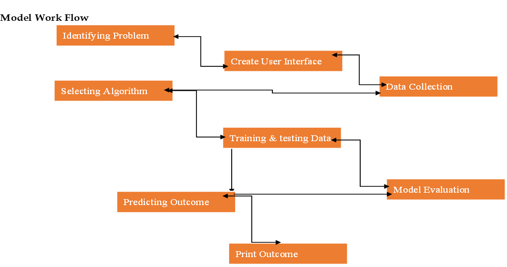
Material and Methodology
A secondary data-set from the Kaggle data platform was used to predict airline passengers’ satisfaction using machine algorithms Random Forest classifier the Datasets were partitioned into training and testing, 70% of the data was retained as a training set while 30% was considered as a testing set.
Read Data File
In this stage the data were reprocessed
# Capd %>% na.omit() # Removing missing values in the dataset
#
# # Converting data types using the following methods below
# Capd$Gender <- as.factor(Capd$Gender)
# Capd$customer_type <-  as.factor(Capd$customer_type)
# Capd$type_of_travel <- as.factor(Capd$type_of_travel)
# Capd$customer_class <- as.factor(Capd$customer_class)
# Capd$flight_distance <- as.integer (Capd$flight_distance)
# Capd$inflight_wifi_service <- as.factor(Capd$inflight_wifi_service)
# Capd$ease_of_online_booking <- as.factor(Capd$ease_of_online_booking)
# Capd$gate_location <- as.factor(Capd$food_and_drink)
# Capd$food_and_drink <- as.factor(Capd$food_and_drink)
# Capd$online_boarding <- as.factor(Capd$online_boarding)
# Capd$seat_comfort <- as.factor(Capd$seat_comfort)
# Capd$inflight_entertainment <- as.factor(Capd$inflight_entertainment)
# Capd$onboard_service <- as.factor(Capd$onboard_service)
# Capd$leg_room_service <- as.factor(Capd$leg_room_service)
# Capd$baggage_handling <- as.factor(Capd$baggage_handling)
# Capd$checkin_service <- as.factor(Capd$checkin_service)
# Capd$inflight_service <- as.factor(Capd$inflight_service)
# Capd$cleanliness <- as.integer (Capd$departure_delay_in_minutes)
# Capd$departure_delay_in_minutes <- as.integer(Capd$departure_delay_in_minutes)
# Capd$arrival_delay_in_minutes <- as.integer(Capd$arrival_delay_in_minutes)
# Capd$satisfaction <- as.factor(Capd$satisfaction)
## Diagram presentation
Table 1: Demo-graphical Characteristics of study participants
| Characteristic | N = 129,8801 |
|---|---|
| Gender | |
| Female | 65,899 (51%) |
| Male | 63,981 (49%) |
| customer_type | |
| disloyal Customer | 23,780 (18%) |
| Loyal Customer | 106,100 (82%) |
| customer_class | |
| Business | 62,160 (48%) |
| Eco | 58,309 (45%) |
| Eco Plus | 9,411 (7.2%) |
| 1 n (%) | |
Capd %>%
  select(age,flight_distance,cleanliness,departure_delay_in_minutes,arrival_delay_in_minutes) %>%
na.omit() %>%  report_parameters()
- age: n = 129487, Mean = 39.43, SD = 15.12, Median = 40.00, MAD = 17.79, range: [7, 85], Skewness = -3.38e-03, Kurtosis = -0.72, 0% missing
- flight_distance: n = 129487, Mean = 1190.21, SD = 997.56, Median = 844.00, MAD = 767.99, range: [31, 4983], Skewness = 1.11, Kurtosis = 0.27, 0% missing
- cleanliness: n = 129487, Mean = 3.29, SD = 1.31, Median = 3.00, MAD = 1.48, range: [0, 5], Skewness = -0.30, Kurtosis = -1.01, 0% missing
- departure_delay_in_minutes: n = 129487, Mean = 14.64, SD = 37.93, Median = 0.00, MAD = 0.00, range: [0, 1592], Skewness = 6.85, Kurtosis = 101.88, 0% missing
- arrival_delay_in_minutes: n = 129487, Mean = 15.09, SD = 38.47, Median = 0.00, MAD = 0.00, range: [0, 1584], Skewness = 6.67, Kurtosis = 95.12, 0% missingtab_xtab(var.row = Capd$Gender,
var.col = Capd$customer_type,
show.row.prc = T)| Gender | customer_type | Total | |
|---|---|---|---|
| disloyal Customer | Loyal Customer | ||
| Female |
12843 19.5 % |
53056 80.5 % |
65899 100 % |
| Male |
10937 17.1 % |
53044 82.9 % |
63981 100 % |
| Total |
23780 18.3 % |
106100 81.7 % |
129880 100 % |
| χ2=124.313 · df=1 · φ=0.031 · p=0.000 | |||
tab_xtab(var.row = Capd$Gender,
         var.col = Capd$type_of_travel,
show.row.prc = T)| Gender | type_of_travel | Total | |
|---|---|---|---|
| Business travel | Personal Travel | ||
| Female |
45794 69.5 % |
20105 30.5 % |
65899 100 % |
| Male |
43899 68.6 % |
20082 31.4 % |
63981 100 % |
| Total |
89693 69.1 % |
40187 30.9 % |
129880 100 % |
| χ2=11.687 · df=1 · φ=0.010 · p=0.001 | |||
tab_xtab(var.row = Capd$Gender,
         var.col = Capd$customer_class,
show.row.prc = T)| Gender | customer_class | Total | ||
|---|---|---|---|---|
| Business | Eco | Eco Plus | ||
| Female |
31263 47.4 % |
29670 45 % |
4966 7.5 % |
65899 100 % |
| Male |
30897 48.3 % |
28639 44.8 % |
4445 6.9 % |
63981 100 % |
| Total |
62160 47.9 % |
58309 44.9 % |
9411 7.2 % |
129880 100 % |
| χ2=20.908 · df=2 · Cramer's V=0.013 · p=0.000 | ||||
Feature Selection
#FS <- Boruta(satisfaction~., data = Capd, doTrace =2)Data Partition in to training and testing
set.seed(1234) # A Random Sampling with replacement

#Data Partition in to trainign and testing

# Model <- sample(2, nrow(Capd), replace = T, prob = c(0.7, 0.3))
# train <- Capd[Model ==1,]
# test <- Capd[Model ==2,]
Building/Developing the models using Decision Tree
# Random Forest Model
# set.seed(333)
# as.data.frame(Capd) # we converted the data in to datafarme
#
# rf23 <-randomForest(satisfaction~., data = train, method = "class", na.action=na.exclude)
Training the Model
# # Prediction & Confusion Matrix - Test
# p <- predict(rf23, train)
# confusionMatrix(p, train$satisfaction)
Evaluating the Model
# p2 <- predict(rf23, test)
# confusionMatrix(p2, test$satisfaction)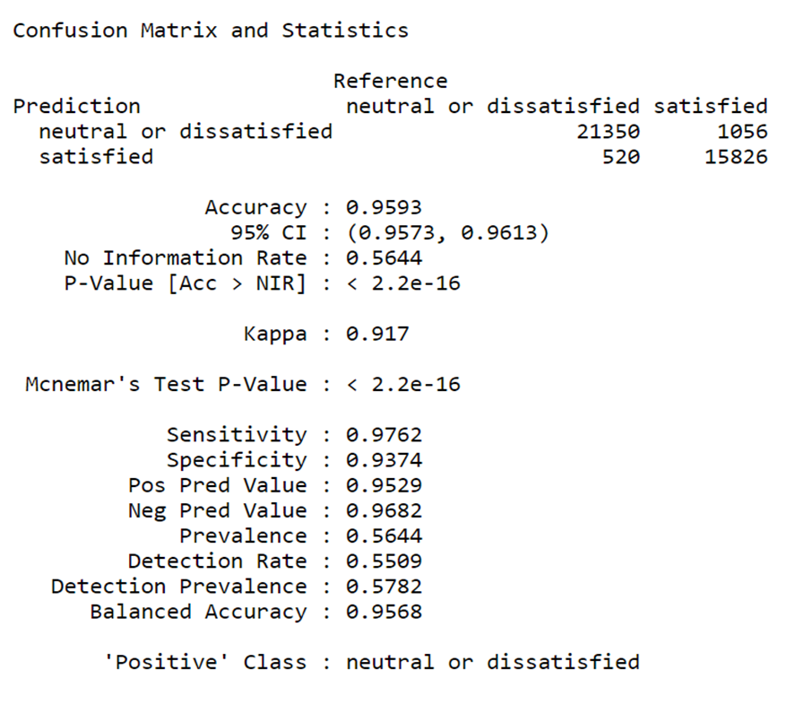
# ConfusionTableR::binary_visualiseR(train_labels = train$satisfaction,
#                                    truth_labels= train$satisfaction,
#                                    class_label1 = "Not satisfied",
#                                    class_label2 = "Satisfied",
#                                    quadrant_col1 = "#28ACB4",
#                                    quadrant_col2 = "#4397D2",
#                                    custom_title = "Confusion Metric on Airline P",
#                                    text_col= "black")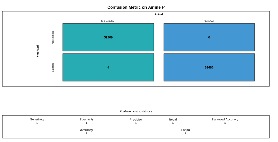
# ConfusionTableR::binary_visualiseR(train_labels = test$satisfaction,
#                                    truth_labels= test$satisfaction,
#                                    class_label1 = "Not satisfied",
#                                    class_label2 = "Satisfied",
#                                    quadrant_col1 = "#28ACB4",
#                                    quadrant_col2 = "#4397D2",
#                                    custom_title = "Confusion Metric on Airline P",
#                                    text_col= "black")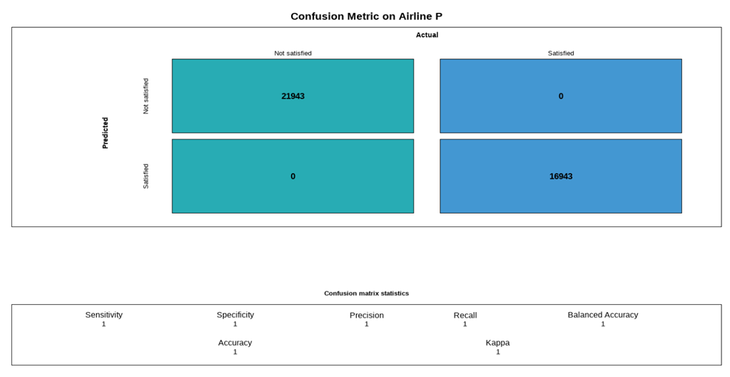
Result
The demographical profiles of the airline passengers; 65899(51%) were females while 63981(49%) were males. Customer class, 62160 (48%) were business class, 58309 (45%) were Economic class and 9411(7.2%) were Economic plus class. The mean age of the airline passengers was 39.4 years with a standard deviation of 15. The average flight distance was 1190.2 miles The overall accuracy of the model was found to be 95% with a sensitivity of 97% and specificity of 93%
Conclusion
Most of the customers were unsatisfied with the airline service. Therefore based on these findings, the Random-Forest algorism predicated 57% at 95% accuracy with a sensitivity of 97% and specificity of 93% that the participants were not satisfied with the daily operation of the airline industry, especially in the areas involved in Air travelers purchasing ticket/booking online, values added services such, In-flight Wi-Fi service check-in in service, Baggage handling, in-flight entertainments, customer service quality, timely departure time, safety, customer service solutions, price, website ease of use.
Recommendation
Considering that 57% of participants reported not being satisfied with airline service rendered this is a significant proportion that may significantly decrease the daily, weekly or monthly income revenues generated. Therefore, this study recommends that the airline industry should endeavor to improve daily operation services, especially in the areas of travelers purchasing tickets/booking online, value-added services such, as In-flight Wi-Fi service, check-in service, Baggage handling, inflight entertainment, customer service quality, timely departure time, safety, customer service solutions, price, website ease of use. This will increase the volume of patronage and, as a result, boost their market share and hence profitability.