In this document we used R to do the automate data analytics using R programming language, an open-source language used for statistical computing and graphics

Hypothesis
H0: There is no significant difference between the Information officers and Industrial workers
H1: There is significant difference between the Information officers and Industrial workers
H0: The salary/wage has no significant influence on education, race, and job-class
H1: The salary/wage has significant influence on education, race, and job-class
Below are the variables we are going to used for this Data Analysis
Table2 Demographic Characteristics
| Characteristic | N = 3,0001 |
|---|---|
| education | |
| 1. < HS Grad | 268 (8.9%) |
| 2. HS Grad | 971 (32%) |
| 3. Some College | 650 (22%) |
| 4. College Grad | 685 (23%) |
| 5. Advanced Degree | 426 (14%) |
| age | 42 (34, 51) |
| health | |
| 1. <=Good | 858 (29%) |
| 2. >=Very Good | 2,142 (71%) |
| 1 n (%); Median (IQR) | |
Table2 Distribution by Marital Status
| Characteristic | N = 3,0001 |
|---|---|
| maritl | |
| 1. Never Married | 648 (22%) |
| 2. Married | 2,074 (69%) |
| 3. Widowed | 19 (0.6%) |
| 4. Divorced | 204 (6.8%) |
| 5. Separated | 55 (1.8%) |
| health_ins | |
| 1. Yes | 2,083 (69%) |
| 2. No | 917 (31%) |
| 1 n (%) | |
Table2 Socio-economic factors
| Characteristic | N = 3,0001 |
|---|---|
| wage | 105 (85, 129) |
| jobclass | |
| 1. Industrial | 1,544 (51%) |
| 2. Information | 1,456 (49%) |
| race | |
| 1. White | 2,480 (83%) |
| 2. Black | 293 (9.8%) |
| 3. Asian | 190 (6.3%) |
| 4. Other | 37 (1.2%) |
| 1 Median (IQR); n (%) | |
| Characteristic | N = 3,0001 |
|---|---|
| region | |
| 1. New England | 0 (0%) |
| 2. Middle Atlantic | 3,000 (100%) |
| 3. East North Central | 0 (0%) |
| 4. West North Central | 0 (0%) |
| 5. South Atlantic | 0 (0%) |
| 6. East South Central | 0 (0%) |
| 7. West South Central | 0 (0%) |
| 8. Mountain | 0 (0%) |
| 9. Pacific | 0 (0%) |
| 1 n (%) | |
| Characteristic | N = 3,0001 |
|---|---|
| year | |
| 2003 | 513 (17%) |
| 2004 | 485 (16%) |
| 2005 | 447 (15%) |
| 2006 | 392 (13%) |
| 2007 | 386 (13%) |
| 2008 | 388 (13%) |
| 2009 | 389 (13%) |
| 1 n (%) | |
Linear regression analysis
Parameter                 | Coefficient |           95% CI | t(2998) |      p | Std. Coef. | Std. Coef. 95% CI |      Fit
-------------------------------------------------------------------------------------------------------------------------
(Intercept)               |      103.32 | [101.28, 105.36] |   99.43 | < .001 |      -0.20 |    [-0.25, -0.15] |
jobclass [2. Information] |       17.27 | [ 14.35,  20.20] |   11.58 | < .001 |       0.41 |    [ 0.34,  0.48] |
                          |             |                  |         |        |            |                   |
AIC                       |             |                  |         |        |            |                   | 30774.50
AICc                      |             |                  |         |        |            |                   | 30774.51
BIC                       |             |                  |         |        |            |                   | 30792.52
R2                        |             |                  |         |        |            |                   |     0.04
R2 (adj.)                 |             |                  |         |        |            |                   |     0.04
Sigma                     |             |                  |         |        |            |                   |    40.83
In this section we used a report function to generate the narrative of binary linear regression
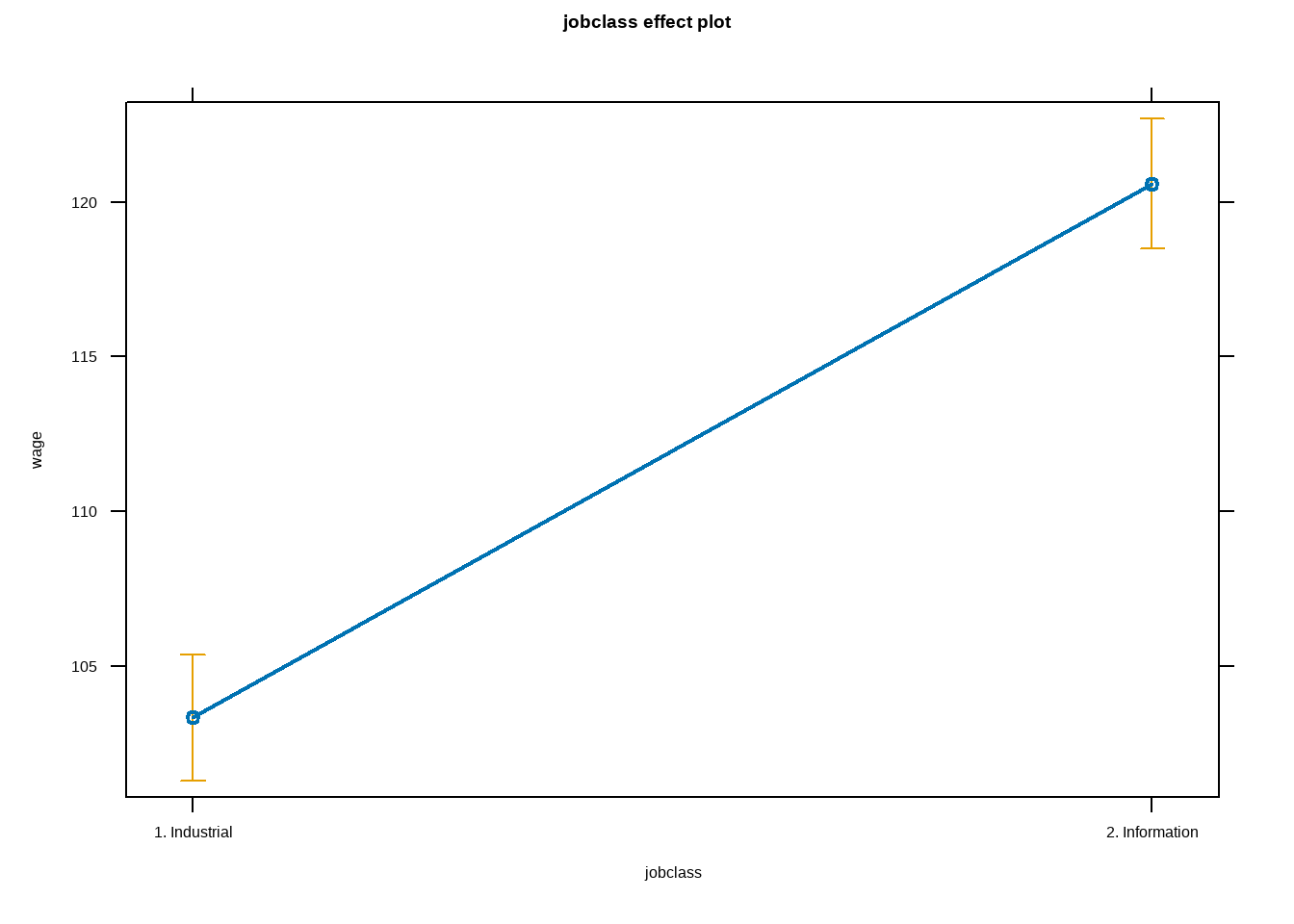
We fitted a linear model (estimated using OLS) to predict wage with jobclass (formula: wage ~ jobclass). The model explains a statistically significant and weak proportion of variance (R2 = 0.04, F(1, 2998) = 134.07, p < .001, adj. R2 = 0.04). The model’s intercept, corresponding to jobclass = 1. Industrial, is at 103.32 (95% CI [101.28, 105.36], t(2998) = 99.43, p < .001). Within this model:
- The effect of jobclass [2. Information] is statistically significant and positive (beta = 17.27, 95% CI [14.35, 20.20], t(2998) = 11.58, p < .001; Std. beta = 0.41, 95% CI [0.34, 0.48])
Standardized parameters were obtained by fitting the model on a standardized version of the dataset. 95% Confidence Intervals (CIs) and p-values were computed using a Wald t-distribution approximation.
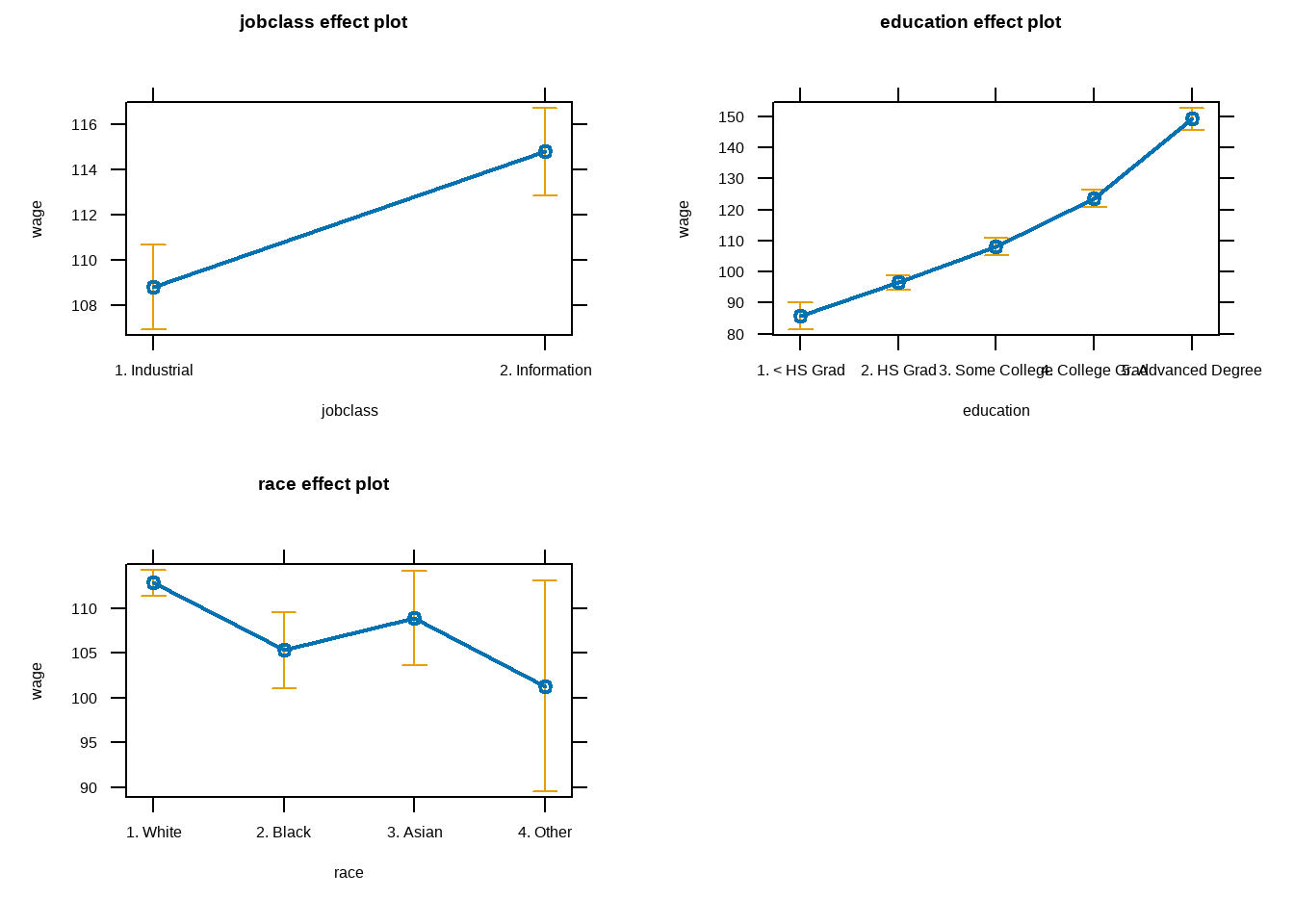
Multiple linear regression
analysis in this model we are going to explore the influence of wage/salary as dependent variables and Age, Race, Education, and Marital status of the employee
Table of multiple logistics regression analysis
| Characteristic | Beta | 95% CI1 | p-value |
|---|---|---|---|
| jobclass | |||
| 1. Industrial | — | — | |
| 2. Information | 6.0 | 3.2, 8.8 | <0.001 |
| education | |||
| 1. < HS Grad | — | — | |
| 2. HS Grad | 11 | 5.9, 16 | <0.001 |
| 3. Some College | 22 | 17, 28 | <0.001 |
| 4. College Grad | 38 | 33, 43 | <0.001 |
| 5. Advanced Degree | 63 | 58, 69 | <0.001 |
| race | |||
| 1. White | — | — | |
| 2. Black | -7.5 | -12, -3.1 | <0.001 |
| 3. Asian | -4.0 | -9.4, 1.5 | 0.2 |
| 4. Other | -12 | -23, 0.33 | 0.057 |
| 1 CI = Confidence Interval | |||
ExpCatViz(
  Wage %>%
    select(education, jobclass),
  target = "education"
  )
[[1]]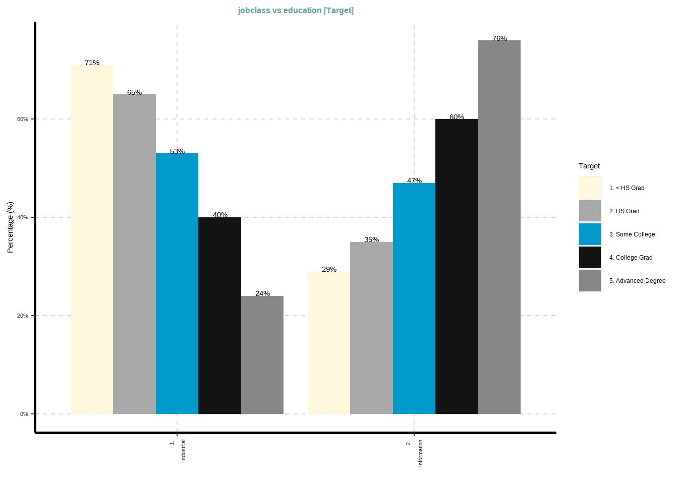
plot_frq(Wage$education)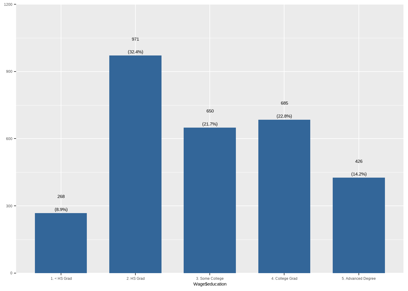
Wage %>%
  group_by(race) %>%
  plot_frq(education) %>%
  plot_grid()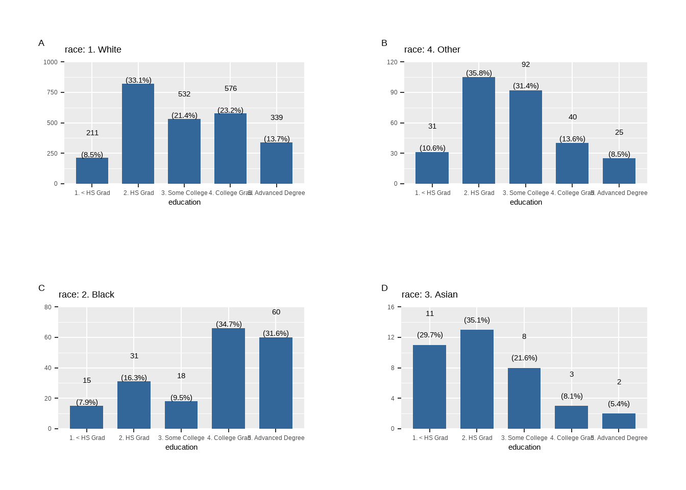
#save_plot(filename = "myplot", fig = p, png, width = 30, height = 19)plot_xtab(x = Wage$education,
grp = Wage$jobclass,
margin = "row",
bar.pos = "stack",
show.summary = T,
coord.flip = T)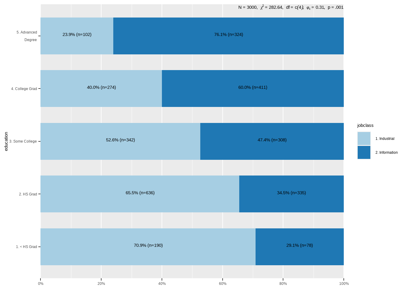
tab_xtab(var.row = Wage$education,
         var.col = Wage$jobclass,
show.row.prc = T)| education | jobclass | Total | |
|---|---|---|---|
| 1. Industrial | 2. Information | ||
| 1. < HS Grad |
190 70.9 % |
78 29.1 % |
268 100 % |
| 2. HS Grad |
636 65.5 % |
335 34.5 % |
971 100 % |
| 3. Some College |
342 52.6 % |
308 47.4 % |
650 100 % |
| 4. College Grad |
274 40 % |
411 60 % |
685 100 % |
| 5. Advanced Degree |
102 23.9 % |
324 76.1 % |
426 100 % |
| Total |
1544 51.5 % |
1456 48.5 % |
3000 100 % |
| χ2=282.643 · df=4 · Cramer's V=0.307 · p=0.000 | |||
Analyses were conducted using the R Statistical language (version 4.3.2; R Core Team, 2023) on Windows 10 x64 (build 19045), using the packages lme4 (version 1.1.35.1; Bates D et al., 2015), Matrix (version 1.6.1.1; Bates D et al., 2023), likert (version 1.3.5; Bryer J, Speerschneider K, 2016), glmulti (version 1.0.8; Calcagno V, 2020), xtable (version 1.8.4; Dahl D et al., 2019), SmartEDA (version 0.3.9; Dayanand Ubrangala et al., 2022), effects (version 4.2.2; Fox J, Weisberg S, 2019), carData (version 3.0.5; Fox J et al., 2022), lubridate (version 1.9.3; Grolemund G, Wickham H, 2011), DiagrammeR (version 1.0.10; Iannone R, 2023), ISLR (version 1.4; James G et al., 2021), lmerTest (version 3.1.3; Kuznetsova A et al., 2017), sjPlot (version 2.8.15; Lüdecke D, 2023), performance (version 0.10.8; Lüdecke D et al., 2021), report (version 0.5.8; Makowski D et al., 2023), e1071 (version 1.7.14; Meyer D et al., 2023), leaps (version 3.1; Miller TLboFcbA, 2020), tibble (version 3.2.1; Müller K, Wickham H, 2023), dlookr (version 0.6.3; Ryu C, 2024), gtsummary (version 1.7.2; Sjoberg D et al., 2021), rJava (version 1.0.11; Urbanek S, 2024), ggplot2 (version 3.4.4; Wickham H, 2016), forcats (version 1.0.0; Wickham H, 2023), stringr (version 1.5.1; Wickham H, 2023), tidyverse (version 2.0.0; Wickham H et al., 2019), dplyr (version 1.1.4; Wickham H et al., 2023), purrr (version 1.0.2; Wickham H, Henry L, 2023), readr (version 2.1.5; Wickham H et al., 2024) and tidyr (version 1.3.1; Wickham H et al., 2024).
References
- Bates D, Mächler M, Bolker B, Walker S (2015). “Fitting Linear Mixed-Effects Models Using lme4.” Journal of Statistical Software, 67(1), 1-48. doi:10.18637/jss.v067.i01 https://doi.org/10.18637/jss.v067.i01.
- Bates D, Maechler M, Jagan M (2023). Matrix: Sparse and Dense Matrix Classes and Methods. R package version 1.6-1.1, https://CRAN.R-project.org/package=Matrix.
- Bryer J, Speerschneider K (2016). likert: Analysis and Visualization Likert Items. R package version 1.3.5, https://CRAN.R-project.org/package=likert.
- Calcagno V (2020). glmulti: Model Selection and Multimodel Inference Made Easy. R package version 1.0.8, https://CRAN.R-project.org/package=glmulti.
- Dahl D, Scott D, Roosen C, Magnusson A, Swinton J (2019). xtable: Export Tables to LaTeX or HTML. R package version 1.8-4, https://CRAN.R-project.org/package=xtable.
- Dayanand Ubrangala, R K, Prasad Kondapalli R, Putatunda S (2022). SmartEDA: Summarize and Explore the Data. R package version 0.3.9, https://CRAN.R-project.org/package=SmartEDA.
- Fox J, Weisberg S (2019). An R Companion to Applied Regression, 3rd edition. Sage, Thousand Oaks CA. https://socialsciences.mcmaster.ca/jfox/Books/Companion/index.html. Fox J, Weisberg S (2018). “Visualizing Fit and Lack of Fit in Complex Regression Models with Predictor Effect Plots and Partial Residuals.” Journal of Statistical Software, 87(9), 1-27. doi:10.18637/jss.v087.i09 https://doi.org/10.18637/jss.v087.i09. Fox J (2003). “Effect Displays in R for Generalised Linear Models.” Journal of Statistical Software, 8(15), 1-27. doi:10.18637/jss.v008.i15 https://doi.org/10.18637/jss.v008.i15. Fox J, Hong J (2009). “Effect Displays in R for Multinomial and Proportional-Odds Logit Models: Extensions to the effects Package.” Journal of Statistical Software, 32(1), 1-24. doi:10.18637/jss.v032.i01 https://doi.org/10.18637/jss.v032.i01.
- Fox J, Weisberg S, Price B (2022). carData: Companion to Applied Regression Data Sets. R package version 3.0-5, https://CRAN.R-project.org/package=carData.
- Grolemund G, Wickham H (2011). “Dates and Times Made Easy with lubridate.” Journal of Statistical Software, 40(3), 1-25. https://www.jstatsoft.org/v40/i03/.
- Iannone R (2023). DiagrammeR: Graph/Network Visualization. R package version 1.0.10, https://CRAN.R-project.org/package=DiagrammeR.
- James G, Witten D, Hastie T, Tibshirani R (2021). ISLR: Data for an Introduction to Statistical Learning with Applications in R. R package version 1.4, https://CRAN.R-project.org/package=ISLR.
- Kuznetsova A, Brockhoff PB, Christensen RHB (2017). “lmerTest Package: Tests in Linear Mixed Effects Models.” Journal of Statistical Software, 82(13), 1-26. doi:10.18637/jss.v082.i13 https://doi.org/10.18637/jss.v082.i13.
- Lüdecke D (2023). sjPlot: Data Visualization for Statistics in Social Science. R package version 2.8.15, https://CRAN.R-project.org/package=sjPlot.
- Lüdecke D, Ben-Shachar M, Patil I, Waggoner P, Makowski D (2021). “performance: An R Package for Assessment, Comparison and Testing of Statistical Models.” Journal of Open Source Software, 6(60), 3139. doi:10.21105/joss.03139 https://doi.org/10.21105/joss.03139.
- Makowski D, Lüdecke D, Patil I, Thériault R, Ben-Shachar M, Wiernik B (2023). “Automated Results Reporting as a Practical Tool to Improve Reproducibility and Methodological Best Practices Adoption.” CRAN. https://easystats.github.io/report/.
- Meyer D, Dimitriadou E, Hornik K, Weingessel A, Leisch F (2023). e1071: Misc Functions of the Department of Statistics, Probability Theory Group (Formerly: E1071), TU Wien. R package version 1.7-14, https://CRAN.R-project.org/package=e1071.
- Miller TLboFcbA (2020). leaps: Regression Subset Selection. R package version 3.1, https://CRAN.R-project.org/package=leaps.
- Müller K, Wickham H (2023). tibble: Simple Data Frames. R package version 3.2.1, https://CRAN.R-project.org/package=tibble.
- R Core Team (2023). R: A Language and Environment for Statistical Computing. R Foundation for Statistical Computing, Vienna, Austria. https://www.R-project.org/.
- Ryu C (2024). dlookr: Tools for Data Diagnosis, Exploration, Transformation. R package version 0.6.3, https://CRAN.R-project.org/package=dlookr.
- Sjoberg D, Whiting K, Curry M, Lavery J, Larmarange J (2021). “Reproducible Summary Tables with the gtsummary Package.” The R Journal, 13, 570-580. doi:10.32614/RJ-2021-053 https://doi.org/10.32614/RJ-2021-053, https://doi.org/10.32614/RJ-2021-053.
- Urbanek S (2024). rJava: Low-Level R to Java Interface. R package version 1.0-11, https://CRAN.R-project.org/package=rJava.
- Wickham H (2016). ggplot2: Elegant Graphics for Data Analysis. Springer-Verlag New York. ISBN 978-3-319-24277-4, https://ggplot2.tidyverse.org.
- Wickham H (2023). forcats: Tools for Working with Categorical Variables (Factors). R package version 1.0.0, https://CRAN.R-project.org/package=forcats.
- Wickham H (2023). stringr: Simple, Consistent Wrappers for Common String Operations. R package version 1.5.1, https://CRAN.R-project.org/package=stringr.
- Wickham H, Averick M, Bryan J, Chang W, McGowan LD, François R, Grolemund G, Hayes A, Henry L, Hester J, Kuhn M, Pedersen TL, Miller E, Bache SM, Müller K, Ooms J, Robinson D, Seidel DP, Spinu V, Takahashi K, Vaughan D, Wilke C, Woo K, Yutani H (2019). “Welcome to the tidyverse.” Journal of Open Source Software, 4(43), 1686. doi:10.21105/joss.01686 https://doi.org/10.21105/joss.01686.
- Wickham H, François R, Henry L, Müller K, Vaughan D (2023). dplyr: A Grammar of Data Manipulation. R package version 1.1.4, https://CRAN.R-project.org/package=dplyr.
- Wickham H, Henry L (2023). purrr: Functional Programming Tools. R package version 1.0.2, https://CRAN.R-project.org/package=purrr.
- Wickham H, Hester J, Bryan J (2024). readr: Read Rectangular Text Data. R package version 2.1.5, https://CRAN.R-project.org/package=readr.
- Wickham H, Vaughan D, Girlich M (2024). tidyr: Tidy Messy Data. R package version 1.3.1, https://CRAN.R-project.org/package=tidyr.