library(readr)
library(DiagrammeR)
library(tidyverse)
library(report)
library(gtsummary)
#library(caret)
library(e1071)
library(sjPlot)
library(performance)
#library(ggstatsplot)
library(SmartEDA)
library(dlookr)
library(lme4)
library(lmerTest)
#library(neuralnet)
#library(DataExplorer)
#library(rpivotTable)
# library(ConfusionTableR)
# library(reshape)
# library(mlbench)
# library(Boruta)
# library(rpart)
# library(rpart.plot)
# library(randomForest)
#library(flextable)
library(readr)
Capd <- read_csv("Capd.csv")Slide Presentation Predicting Airline Passenger Satisfaction using Random Forest Algorithm
Outline
What is Random Forest Algorithm?
Benefits of Random Forest Algorithm
Predicting Airline Passenger Satisfaction using
Random Forest Algorithm
List of Packages used
Material and Methodology
A secondary data-set from the Kaggle data science platform
Machine algorithms Random Forest classifier
Data sets were partitioned into training and testing,
Of which 70% of the data was retained as a training set while 30% was considered as a testing set.
What is Random Forest Algorithm?
What is Random Forest Algorithm?

What is Random Forest Algorithm?
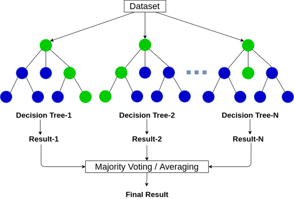
Random Forest Algorithm is an ensemble learning method for classification and regression
Combines multiple decision trees to create a more accurate and stable prediction
Uses bagging and feature randomness when building each individual tree
Benefits of Random Forest Algorithm
- High accuracy and robustness
- Handles missing values and outliers
- Reduces variance compared to a single decision tree
Predicting Airline Passenger Satisfaction

Collect data on airline passengers
Use the Random Forest Algorithm to build a model
Use the model to predict passenger satisfaction
Reading the Data File
Pre-processing
# Capd %>% na.omit() # Removing missing values in the dataset
#
# # Converting data types using the following methods below
# Capd$Gender <- as.factor(Capd$Gender)
# Capd$customer_type <-  as.factor(Capd$customer_type)
# Capd$type_of_travel <- as.factor(Capd$type_of_travel)
# Capd$customer_class <- as.factor(Capd$customer_class)
# Capd$flight_distance <- as.integer (Capd$flight_distance)
# Capd$inflight_wifi_service <- as.factor(Capd$inflight_wifi_service)
# Capd$ease_of_online_booking <- as.factor(Capd$ease_of_online_booking)
Demo-graphical Characteristics
| Characteristic | N = 129,8801 |
|---|---|
| Gender | |
| Female | 65,899 (51%) |
| Male | 63,981 (49%) |
| customer_type | |
| disloyal Customer | 23,780 (18%) |
| Loyal Customer | 106,100 (82%) |
| customer_class | |
| Business | 62,160 (48%) |
| Eco | 58,309 (45%) |
| Eco Plus | 9,411 (7.2%) |
| 1 n (%) | |
Estimated Parameters
Capd %>%
  select(age,flight_distance,cleanliness,departure_delay_in_minutes,arrival_delay_in_minutes) %>%
na.omit() %>%  report_parameters()
- age: n = 129487, Mean = 39.43, SD = 15.12, Median = 40.00, MAD = 17.79, range: [7, 85], Skewness = -3.38e-03, Kurtosis = -0.72, 0% missing
- flight_distance: n = 129487, Mean = 1190.21, SD = 997.56, Median = 844.00, MAD = 767.99, range: [31, 4983], Skewness = 1.11, Kurtosis = 0.27, 0% missing
- cleanliness: n = 129487, Mean = 3.29, SD = 1.31, Median = 3.00, MAD = 1.48, range: [0, 5], Skewness = -0.30, Kurtosis = -1.01, 0% missing
- departure_delay_in_minutes: n = 129487, Mean = 14.64, SD = 37.93, Median = 0.00, MAD = 0.00, range: [0, 1592], Skewness = 6.85, Kurtosis = 101.88, 0% missing
- arrival_delay_in_minutes: n = 129487, Mean = 15.09, SD = 38.47, Median = 0.00, MAD = 0.00, range: [0, 1584], Skewness = 6.67, Kurtosis = 95.12, 0% missingCross-Tabulation of Customers Type
| Gender | customer_type | Total | |
|---|---|---|---|
| disloyal Customer | Loyal Customer | ||
| Female | 12843 19.5 % |
53056 80.5 % |
65899 100 % |
| Male | 10937 17.1 % |
53044 82.9 % |
63981 100 % |
| Total | 23780 18.3 % |
106100 81.7 % |
129880 100 % |
| χ2=124.313 · df=1 · φ=0.031 · p=0.000 | |||
Cross-Tabulation based on Class
| Gender | customer_class | Total | ||
|---|---|---|---|---|
| Business | Eco | Eco Plus | ||
| Female | 31263 47.4 % |
29670 45 % |
4966 7.5 % |
65899 100 % |
| Male | 30897 48.3 % |
28639 44.8 % |
4445 6.9 % |
63981 100 % |
| Total | 62160 47.9 % |
58309 44.9 % |
9411 7.2 % |
129880 100 % |
| χ2=20.908 · df=2 · Cramer's V=0.013 · p=0.000 | ||||
Conceptual Model used

Feature Selection
Data Partition
Building the Model
Training set of the Model
Training set of the Model
Testing Set of the Model
Testing Set of the Model
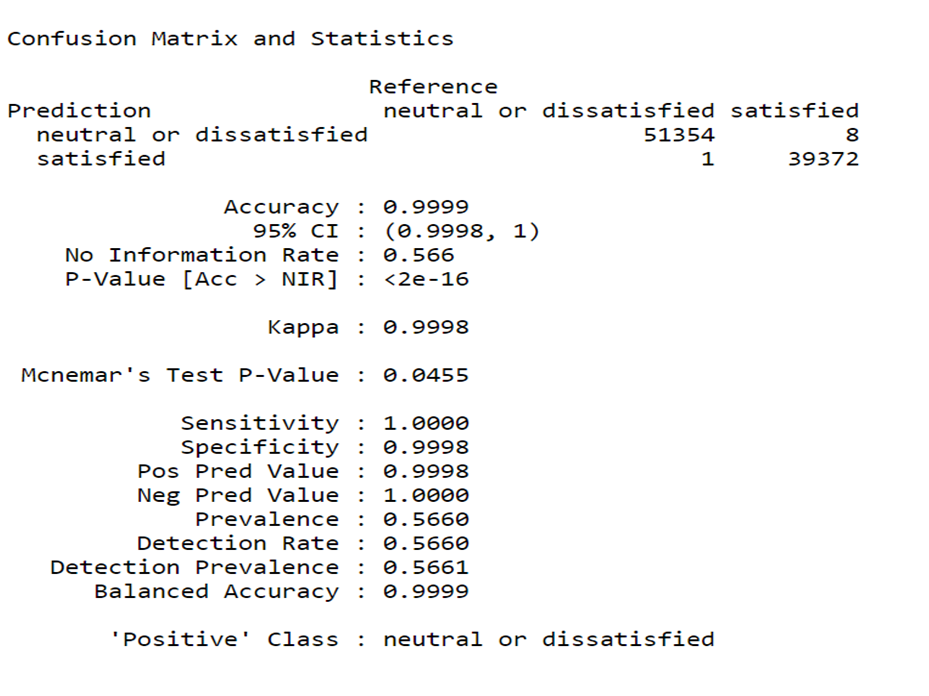
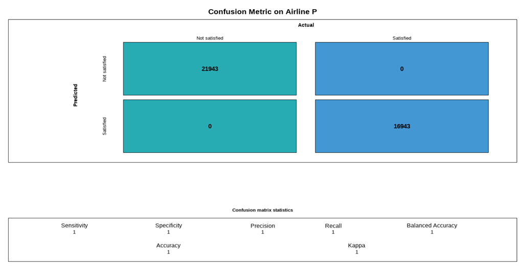
Confusion Metrix for Training set
# ConfusionTableR::binary_visualiseR(train_labels = train$satisfaction,
#                                    truth_labels= train$satisfaction,
#                                    class_label1 = "Not satisfied",
#                                    class_label2 = "Satisfied",
#                                    quadrant_col1 = "#28ACB4",
#                                    quadrant_col2 = "#4397D2",
#                                    custom_title = "Confusion Metric on Airline P",
#                                    text_col= "black")
Confusion Metrix for Training set

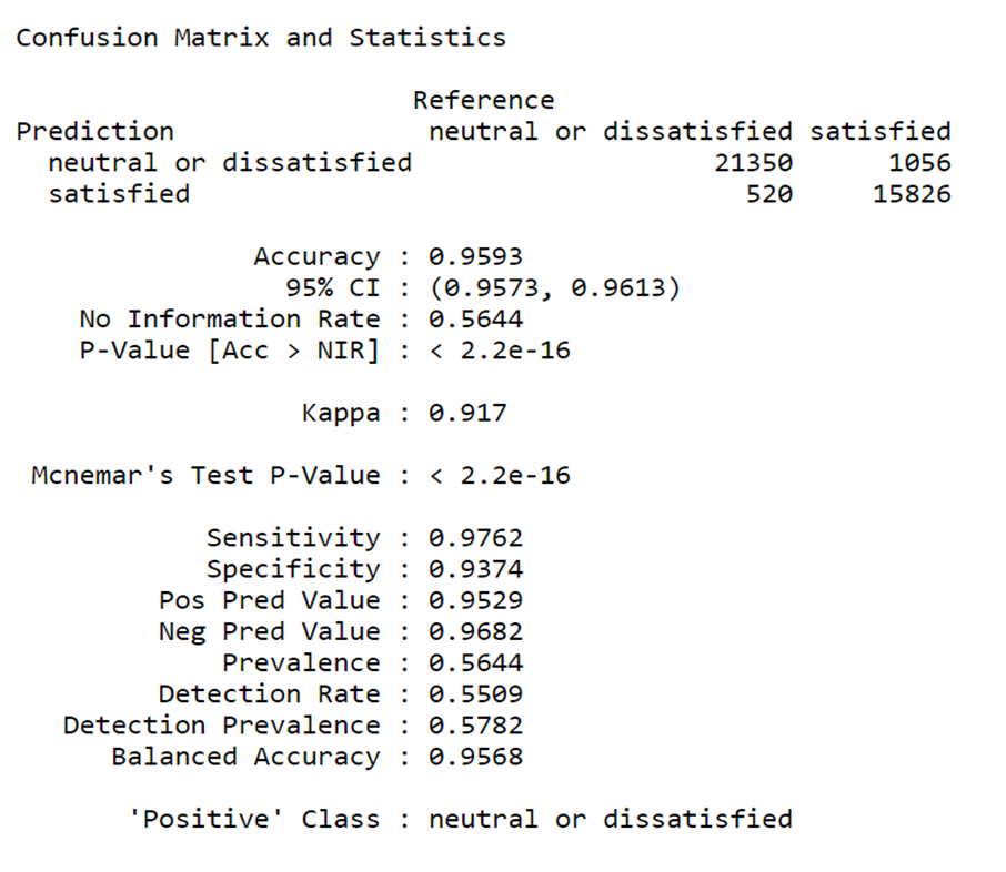
Confusion Metrix for Testing set
Confusion Metrix for Testing set
Conclusion
The overall accuracy of the model was found to be 95% with a sensitivity of 97% and specificity of 93%
Most of the customers were unsatisfied with the airline service. Therefore based on these findings, the Random-Forest algorism predicated 57% at 95% accuracy with a sensitivity of 97% and specificity of 93% that the participants were not satisfied with the daily operation of the airline industry, especially in the areas involved in Air travelers purchasing ticket/booking online, values added services
Recommendation
Considering that 57% of participants reported not being satisfied with airline service rendered this is a significant proportion that may significantly decrease the daily, weekly or monthly income revenues generated.
Therefore, this findings recommends that the airline industry should endeavor to improve daily operation services, especially in the areas of travelers purchasing tickets/booking online, value-added services such, as In-flight Wi-Fi service, check-in service, Baggage handling
This will increase the volume of patronage and, as a result, boost their market share and hence profitability.